The Tooling System: 50+ Tools, One Registry, and How Schema Weaver's Data Explorer Actually Executes Work
An agent loop without tools is just a chatbot. Schema Weaver's Data Explorer ships with 50+ tools across 10 functional phases — from database exploration to predictive modeling and AI self-management. Each tool follows a standardized contract, executes through a secure read-only proxy, compresses results through a 3-tier context limiter, and emits interactive artifacts. Here is the complete tooling system — the registry, the security boundaries, the execution pipeline, and the artifact mapping that makes the agent's work visible to users. Part 3 of the Data Explorer Architecture Deep Dive
In Part 2, we showed how Schema Weaver's Data Explorer runs a single LLM in a ReAct loop — one model, one conversation, up to 15 iterations. But a reasoning loop without tools is just a chatbot. The real work happens when the agent calls tools. This is the part most architecture blogs skip — they show you the agent loop, then hand-wave the tooling. We won't do that here.
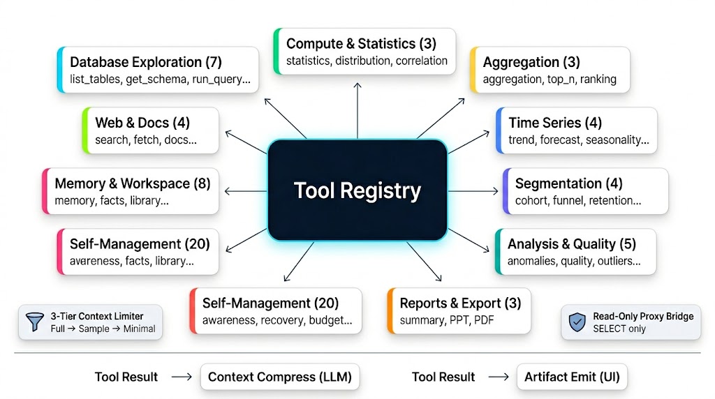
Schema Weaver Data Explorer ships with 50+ tools organized across 10 functional phases — from basic database exploration to predictive modeling, report generation, and AI self-management. Each tool follows a standardized contract: schema declaration, execution, result formatting, and artifact emission. Every tool call goes through a secure Node.js proxy that enforces read-only access. Every result passes through a 3-tier context limiter that prevents the LLM from drowning in raw data. And every data-producing tool maps to a specific artifact type that the frontend knows how to render.
This is the complete tooling system — how tools are registered, how they execute, how results flow back to both the LLM and the user interface, and the security boundaries that keep production databases safe while an AI agent runs arbitrary queries against them.
1. Tool Registry Architecture
All tools are registered at startup via create_registry() in a centralized ToolRegistry. The registry is not just a list — it coordinates schema representation for the LLM, access control for execution, parallel query dispatch, context compression, and front-end rendering hints. Every tool call in the agent loop flows through this single entry point.
When the LLM decides to call a tool, the agent loop parses the function call, looks up the tool in the registry, executes it (potentially through the Node.js proxy for database access), compresses the result text for the LLM context, and emits structured events to the frontend for rendering. The LLM never sees the full data. The user always sees the full data. That separation is the core design principle.
1.1 Tool Catalog Overview
The registry indexes 50+ tools categorized across 10 functional phases. This categorization matters because of the intent classification system we covered in Part 2 — when the LLM classifies a user query as "explore", only the database exploration tools get loaded into the schema. When it classifies as "analyze", the compute and analytics tools unlock. The phase structure is the backbone of the 89% token reduction.
This is the full tool catalog. Try it yourself at data-explorer.schemaweaver.vivekmind.com — connect your PostgreSQL database and ask a question. The agent will pick the right tools from this registry automatically.
1.2 The BaseTool Contract
Every tool extends BaseTool and implements three properties and one method. This contract is what makes the registry work — because every tool looks the same to the executor, the system can dispatch, retry, log, and compress results without knowing what the tool actually does.
class BaseTool(ABC):
    @property
    @abstractmethod
    def name(self) -> str:
        """Unique tool name used in LLM function-calling."""

    @property
    @abstractmethod
    def description(self) -> str:
        """Natural language description for the LLM."""

    @property
    @abstractmethod
    def parameters(self) -> list[ToolParameter]:
        """Typed parameter definitions."""

    @abstractmethod
    async def execute(self, *, user_id: str, **kwargs) -> ToolResult:
        """Execute the tool and return a ToolResult."""
The ToolParameter dataclass defines the schema for each parameter. This is what gets converted into the function-calling schema that the LLM sees:
@dataclass
class ToolParameter:
    name: str
    type: str          # "string", "integer", "number", "boolean", "array", "object"
    description: str
    required: bool = True
    default: Any = None
    enum: list = None
    items: dict = None  # For array types
1.3 ToolResult
Every tool returns a standardized ToolResult. Success or failure, the shape is the same. This makes error handling consistent — the agent loop doesn't need special cases for different tools failing in different ways.
@dataclass
class ToolResult:
    status: ToolStatus   # "success" | "error"
    data: dict | None     # Result payload
    error: str | None     # Error message (only on failure)

    @classmethod
    def ok(cls, data: dict) -> ToolResult:
        return cls(status=ToolStatus.SUCCESS, data=data, error=None)

    @classmethod
    def fail(cls, error: str) -> ToolResult:
        return cls(status=ToolStatus.ERROR, data=None, error=error)
1.4 Schema Generation for LLMs
The registry generates OpenAI-compatible function-calling schemas for all tools. This is the JSON that gets injected into the LLM request as tools. The intent classification system from Part 2 controls which of these schemas actually get sent — that's how we go from 50+ tool schemas (18K tokens) to only the relevant ones (2K tokens).
def to_schema(self) -> dict:
    return {
        "type": "function",
        "function": {
            "name": self.name,
            "description": self.description,
            "parameters": {
                "type": "object",
                "properties": {
                    p.name: {"type": p.type, "description": p.description}
                    for p in self.parameters
                },
                "required": [p.name for p in self.parameters if p.required],
            },
        },
    }
These schemas are then converted to Anthropic/Gemini formats by the provider adapters when the LLM route points to a non-OpenAI model. The tool execution layer stays format-agnostic — it only sees ToolResult objects regardless of which provider handled the call.
1.5 Secure Database Proxy Model (The Bridge)
This is the most important security boundary in the entire system. The Python execution loop — where the agent runs, where tool code executes — does not have direct access or credentials to target databases. Instead, all database-accessing tools run queries through a secure Node.js REST API proxy bridge. The Python sandbox is exactly that: a sandbox. It can make HTTP requests to the bridge, but it cannot connect to PostgreSQL directly.
2. Block writes (INSERT, UPDATE, DELETE)
3. Block transactions (COMMIT, ROLLBACK) alt Validation Failed Bridge-->>Tool: HTTP 403 Forbidden / 400 Invalid Query else Validation Succeeded Bridge->>DB: Execute SELECT query (read-only session) DB-->>Bridge: Result rows Bridge-->>Tool: JSON payload (rows, columns, rowCount) end
The bridge implements three security layers that operate before any query touches the database:
- Connection Ownership — Verifies that the active request session corresponds to the owner of the requested
connection_id. One user's agent cannot query another user's database. This is checked at the API layer, not in the Python sandbox. - Read-Only SELECT Enforcement — Rejects any non-SELECT statements at the API layer. Command strings containing write actions (
INSERT,UPDATE,DELETE,DROP) or transaction indicators (COMMIT,ROLLBACK) are blocked immediately. The agent can never modify data, even if the LLM hallucinates a destructive query. - Result Size Limits — Enforces hard limits (defaulting to 2,000 rows) at the Node.js backend to prevent memory exhaustion in the Python agent container. Even if a user asks "show me everything", the bridge caps the result before it reaches the sandbox.
Why a separate Node.js layer instead of filtering in Python? Because the Python sandbox is controlled by the LLM's output. If the LLM produces unexpected code or the sandbox is compromised, the database is still protected by a separate service that the agent cannot bypass. Defense in depth — the Node.js bridge is the security boundary, not the Python code.
1.6 LLM Context Compression (The 3-Tier Context Limiter)
When a query tool returns data — say 500 rows — the full result is sent to the client to construct the interactive frontend table. Users need to see their data. However, sending the entire raw JSON payload to the LLM would quickly exhaust its context window and inflate token costs. This is the problem we solved with the artifact system in Part 2: the user sees everything, the LLM sees only what it needs to reason.
To make this concrete, Schema Weaver routes all query and data results through a 3-Tier Context Limiter (context_limiter.py), which formats the result text based on total size:
Result Size (Rows)
├── Tier 1 (≤20 rows)     --> Show all rows fully
├── Tier 2 (21-1000 rows)  --> Show first 10 rows + auto-computed column averages/min/max
└── Tier 3 (>1000 rows) --> Show first 3 rows + warnings to use LIMIT/WHERE filters| Tier | Row Count | What the LLM receives | Why |
|---|---|---|---|
| Tier 1 | ≤ 20 rows | Complete dataset | Small enough to fit in context without compression |
| Tier 2 | 21 – 1,000 | 10-row sample + column averages/min/max | Statistical summary enables accurate reasoning without raw data |
| Tier 3 | > 1,000 | 3-row structural sample + column list + filter warning | Forces the agent to generate targeted queries with LIMIT/WHERE |
Tier 1 is straightforward — 20 rows fit comfortably in any model's context window. Tier 2 is where it gets interesting. Instead of dumping 500 rows, the LLM gets a 10-row sample to inspect data formats and values, accompanied by a quick statistical summary of numeric fields (e.g., amount: avg=150, min=15, max=2500). This enables accurate mathematical reasoning without feeding raw data into the context. Tier 3 is the hard stop — the LLM receives only a 3-row structural sample, column lists, and a notice prompting it to generate queries with specific LIMIT or WHERE clauses. The agent is forced to be precise rather than lazy.
This is why we said in Part 2 that raw data never enters the LLM context. The 3-tier limiter is the enforcement mechanism. The artifact system is the delivery mechanism. Together, they solve both privacy and cost — the user sees their full data rendered as tables and charts, while the LLM only sees what it needs to continue reasoning.
1.7 Output Taxonomy: Exploratory Cards vs. Rich Artifacts
Not every tool call deserves screen real estate. Tools are split into two categories based on how they report results to the user interface:
- System/Exploratory Tool Cards — Tools like
list_tables,get_schema, andsample_rowsare intermediate steps used by the agent to acquire metadata. They are rendered only as small progress cards in the conversation timeline to minimize clutter. The user sees "the agent looked at your schema" — they don't need to see the full schema dump in the chat. - Interactive Rich Artifacts — Tools that generate final charts, aggregated tables, or structured summaries (e.g.,
run_query,compute_trend,generate_summary_report) emit full artifact payloads. The frontend intercepts these payloads to create full-tab interactive previews — sortable data tables, line/bar charts, heatmaps, and funnel diagrams that the user can explore.
This distinction is deliberate. If every tool call produced an artifact, the UI would be unusable — a wall of intermediate results drowning out the actual analysis. Exploratory tools are the agent's eyes. Artifact-producing tools are the agent's answers. The user only needs to see the answers.
2. Database Exploration Tools
These are the foundational tools that give the agent eyes into the database. Almost every conversation starts with one or more of these — the agent needs to understand the data landscape before it can analyze anything.
2.1 list_tables
Purpose: Discover all tables in the connected database.
Why it exists: The agent needs to know what data is available before it can do anything else. This is almost always the first tool called in a new session. Without it, the LLM would be guessing table names — and guessing in SQL is how you get hallucinated queries.
// Example tool call from LLM
{
    "name": "list_tables",
    "arguments": {
        "connection_id": "conn_abc123",
        "schema_name": "public"
    }
}
// Example response
{
"tables": [
{"name": "users", "estimatedRows": 15000, "sizeFormatted": "2.1 MB", "hasIndexes": true},
{"name": "orders", "estimatedRows": 48000, "sizeFormatted": "8.5 MB", "hasIndexes": true},
{"name": "products", "estimatedRows": 320, "sizeFormatted": "128 kB", "hasIndexes": true},
{"name": "reviews", "estimatedRows": 12000, "sizeFormatted": "1.8 MB", "hasIndexes": false}
],
"count": 4
}Security: Calls the Node.js backend via GET /api/service/data/{connectionId}/tables. The Node.js layer validates that the authenticated user owns this connection.
2.2 get_schema
Purpose: Get detailed column definitions, types, keys, and indexes for a table.
Why it exists: The agent MUST know exact column names and types before writing any SQL. This prevents the #1 cause of SQL hallucination — wrong column names. If the LLM thinks the column is user_id but it's actually userId, every query downstream fails. get_schema eliminates this class of error entirely.
// Example response
{
    "table": "orders",
    "schema": "public",
    "columns": [
        {"name": "id", "type": "uuid", "nullable": false, "isPrimaryKey": true},
        {"name": "user_id", "type": "uuid", "nullable": false, "isForeignKey": true},
        {"name": "total_amount", "type": "numeric(10,2)", "nullable": false},
        {"name": "status", "type": "varchar(50)", "nullable": false},
        {"name": "created_at", "type": "timestamptz", "nullable": false}
    ],
    "primaryKey": ["id"],
    "indexes": [
        {"name": "idx_orders_user_id", "columns": ["user_id"]},
        {"name": "idx_orders_created_at", "columns": ["created_at"]}
    ]
}
There is a critical rule baked into the system prompt:
"NEVER guess column names. If the table schema is not in your immediate conversation history, ALWAYS call get_schema first."
This single rule prevents the majority of SQL errors in the agent's output. The LLM is forced to verify before it writes, not after.
2.3 run_query
Purpose: Execute a validated read-only SELECT query against the database.
Why it exists: The SQL escape hatch. When no specialized tool covers the user's request, run_query allows arbitrary SELECT statements. This is the most powerful and most dangerous tool — powerful because it can answer any queryable question, dangerous because it relies on the LLM generating correct SQL.
// Example tool call
{
    "name": "run_query",
    "arguments": {
        "connection_id": "conn_abc123",
        "sql": "SELECT status, COUNT(*) as cnt FROM orders GROUP BY status ORDER BY cnt DESC",
        "limit": 100
    }
}
// Example response
{
"sql": "SELECT status, COUNT(*) as cnt FROM orders GROUP BY status ORDER BY cnt DESC",
"rows": [
{"status": "completed", "cnt": 28500},
{"status": "pending", "cnt": 12300},
{"status": "cancelled", "cnt": 7200}
],
"rowCount": 3,
"columns": [{"name": "status"}, {"name": "cnt"}],
"executionMs": 42,
"truncated": false
}Security considerations:
- Only SELECT statements are allowed — the Node.js backend rejects any write operations
- Results are capped at 2,000 rows maximum
- The query runs through the same Node.js proxy that validates connection ownership
- Dangerous query patterns (Cartesian joins, unconstrained aggregations on massive tables) are detected and blocked at the backend level
2.4 sample_rows
Purpose: Fetch a small sample of actual data to understand value formats and distributions.
Why it exists: Schema tells you column names and types, but not what the data actually looks like. Sample rows let the agent understand value formats — are dates stored as ISO strings or Unix timestamps? Are prices in cents or dollars? Is the status field lowercase or Title Case? This context is essential for writing correct SQL.
Limit: Maximum 50 rows, default 20. Deliberately small — this is a reconnaissance tool, not a data export tool.
2.5 count_rows
Purpose: Fast row count with optional WHERE filter.
Why it exists: Faster than run_query for pure count operations. Supports filtered counts like "how many orders are pending?" without the overhead of constructing a full SQL query and parsing the result.
2.6 get_column_stats
Purpose: Statistical summary of all columns — null rates, distinct counts, min/max, sample values.
Why it exists: Gives the agent a quick overview of data quality and distribution before running detailed analysis. If a column has 80% nulls, the agent knows to skip it or flag it. If a column has only 3 distinct values, the agent knows it's categorical. This pre-analysis step prevents wasted iterations on bad data.
2.7 search_rows
Purpose: Filter rows using a structured filter API instead of raw SQL.
// Example tool call
{
    "name": "search_rows",
    "arguments": {
        "connection_id": "conn_abc123",
        "table_name": "orders",
        "filters": [
            {"column": "status", "operator": "eq", "value": "pending"},
            {"column": "total_amount", "operator": "gt", "value": 100}
        ],
        "limit": 50
    }
}
Supported operators: eq, neq, gt, gte, lt, lte, like, is_null, not_null
This tool exists as a safer alternative to run_query for simple filtering. The structured filter API is harder to get wrong than raw SQL, and the Node.js bridge can validate the filter structure more easily than validating freeform SQL.
3. Compute & Analytics Tools
These tools produce rich analytical outputs with automatic chart/stat block artifact generation. They are the reason users come to Schema Weaver's Data Explorer — not just to ask "what tables do I have?" but to get real analytical answers with visual outputs.
3.1 compute_statistics
Computes descriptive statistics for numeric columns: mean, median, std, percentiles (p25/p50/p75/p95), skewness, kurtosis. Produces a stat block artifact — a card-based layout showing each metric with color-coded severity indicators.
3.2 compute_distribution
Computes value distribution (histogram buckets) for a column. Produces a bar chart artifact. Useful for understanding the shape of data — are sales normally distributed? Are there bimodal patterns in user engagement?
3.3 compute_correlation
Computes Pearson correlation between numeric columns. Produces a heatmap artifact with the correlation matrix. When a user asks "what factors influence revenue?", this tool answers it visually — the heatmap immediately highlights strong positive and negative correlations.
3.4 compute_aggregation
GROUP BY with flexible aggregation functions (SUM, AVG, COUNT, MIN, MAX). Produces a bar chart artifact. This is the workhorse tool — most analytical questions boil down to "group by X, aggregate Y".
3.5 compute_top_n
Top N values by a metric column. Produces a ranked bar chart artifact. "Who are our top 10 customers?" — this tool, one call, visual answer.
3.6 compute_trend
Time-series trend analysis with slope detection and direction classification (up/down/flat/volatile). Produces a line chart artifact. The agent doesn't just plot the data — it computes the slope, determines if the trend is statistically meaningful, and reports the direction and magnitude in the tool result. The LLM can then explain the trend to the user in natural language without guessing.
3.7 forecast_trend
Extends compute_trend with future predictions using linear extrapolation and confidence intervals. Produces a line chart with historical data, forecast line, and confidence bands. This is the closest the system gets to predictive modeling — it's deliberately simple (linear extrapolation, not deep learning) because the goal is fast, interpretable predictions that a user can verify, not black-box forecasts.
3.8 compute_cohort
Cohort analysis based on a signup/first-action date. Produces a heatmap artifact showing retention by cohort period. Standard SaaS analytics — "of the users who signed up in January, what percentage were still active in February? March?"
3.9 compute_funnel
Conversion funnel analysis with step-by-step drop-off rates. Produces a funnel chart artifact. The agent identifies each step in the funnel, computes absolute and percentage drop-off, and surfaces the biggest leakage points.
3.10 detect_anomalies
Statistical anomaly detection using Z-score or IQR methods. Produces a stat block artifact listing anomalies by severity. Not machine learning — just statistical methods that work reliably and are explainable to the user.
3.11 check_quality
Data quality scoring (0-100) with issue detection: null rates, duplicates, format inconsistencies. Produces a quality stat block artifact. This tool often runs first when a user connects a new database — it gives the agent a baseline understanding of data quality before any analysis begins.
4. Report Generation Tools
4.1 generate_summary_report
The most complex tool in the system. It takes results from prior analysis tools and generates a structured multi-section report. This is not a template filler — the tool receives actual analytical results and produces a narrative report with executive summaries, key findings, and actionable insights.
Workflow (as specified in the system prompt):
Step 1: Run analysis tools (compute_trend, compute_statistics, etc.)
Step 2: Call generate_summary_report with prior_tool_results
Step 3: Optionally call generate_ppt or generate_pdf
// Example tool call
{
"name": "generate_summary_report",
"arguments": {
"title": "Customer Retention Analysis Q1 2026",
"prior_tool_results": [
{
"tool_name": "compute_retention",
"artifact_type": "retention",
"data": {"matrix": [...], "periods": [...]}
},
{
"tool_name": "compute_trend",
"artifact_type": "trend",
"data": {"direction": "down", "slope": -0.023}
}
]
}
}// Example response
{
"title": "Customer Retention Analysis Q1 2026",
"generatedAt": "2026-05-26T10:00:00Z",
"sections": [
{
"heading": "Executive Summary",
"text": "Customer retention shows a declining trend of -2.3% per period..."
},
{
"heading": "Retention Matrix",
"text": "Day-1 retention is 45%, dropping to 22% by day-30..."
}
],
"insights": [
"D1 retention is above industry average but D7 shows significant drop-off",
"Consider investigating the onboarding flow between day 1 and day 7"
]
}4.2 generate_ppt / generate_pdf
Export tools that convert a summary report into downloadable file formats. These tools take the output of generate_summary_report as input, generate the file server-side, and return a download URL as a file artifact. The user gets a polished document they can share — the full pipeline from natural language question to executive-ready report, no manual formatting required.
5. Self-Management Tools
This is the part most agent systems don't build. Schema Weaver's Data Explorer has 20 self-management tools organized in 6 categories. These give the agent metacognitive abilities — awareness of its own state, ability to track progress, and mechanisms for graceful error handling. An agent without self-management tools is like a developer without a debugger — it can write code, but it can't fix its own mistakes.
| Category | Tools | What it enables |
|---|---|---|
| Self-Awareness | get_run_status, get_tool_history, list_available_tools | Agent knows where it is, what it's done, what it can do |
| Communication | emit_progress, ask_clarification, emit_partial_result | User sees progress in real-time, agent can ask for help |
| Task Tracking | create_task_plan, update_task_step, get_task_plan | Multi-step analysis stays organized and trackable |
| Error Recovery | report_tool_failure, try_fallback, mark_as_unanswerable, get_failed_tools_summary | Graceful failure instead of infinite retry loops |
| Budget Management | get_budget_status, estimate_token_size, compact_working_memory, inject_context | Agent manages its own context window and iteration budget |
| Checkpoints | save_checkpoint, load_checkpoint, clear_checkpoint | Long analyses can be paused and resumed |
The most critical category is Error Recovery. Without it, an agent that hits a bad SQL query will retry the same broken query in a loop, burning through all 15 iterations without progress. With error recovery tools, the agent can: report the failure, try a different approach (e.g., switch from run_query to search_rows with a simpler filter), or mark the question as unanswerable and explain why. This turns infinite loops into graceful degradation — the user gets an honest "I couldn't answer this" instead of 15 iterations of garbage.
Budget Management is equally important. The agent can check how many iterations it has left, estimate the token cost of a tool call before making it, and compact its working memory to free up context for remaining steps. This is self-preservation — the agent actively manages its own resource constraints instead of blindly executing until it hits the 15-iteration wall.
6. Tool-to-Artifact Mapping
Every data-producing tool maps to a specific artifact type, which maps to a specific frontend renderer. This mapping is hardcoded — the frontend doesn't guess what to render. It receives an artifact event with a type field and dispatches to the correct renderer.
Exploratory tools (list_tables, get_schema, sample_rows) deliberately do NOT produce artifacts. They appear only as tool cards in the chat timeline. This prevents the UI from being cluttered with intermediate discovery results — the user sees "the agent checked your schema" as a small card, not a full-screen schema dump.
7. Tool Execution Flow — Complete Pipeline
This is the full sequence — from the LLM deciding to call a tool to the user seeing the rendered result. Every tool call follows this path, whether it's a simple count_rows or a complex generate_summary_report.
seen tool keys"} INJECT["Inject result into
updated context"] end subgraph "Tool Executor" PAR["Execute tools
in parallel"] RECORD["Record + Format
result for LLM"] RETRY{"Retry if failed
and retryable?"} end subgraph "Tool Registry" REG["Dispatch to
tool instance"] end subgraph "Individual Tool" TOOL["Run tool logic"] COMPUTE["Compute analysis
direction + slope"] end subgraph "Node.js Backend" BACK["Validate + Execute
read-only query"] end subgraph "Database" DB[("PostgreSQL")] end subgraph "Artifact Emitter" ART["Build chart artifact
line chart for trend"] end subgraph "SSE Stream" SSE1["status - executing"] SSE2["tool_call event"] SSE3["tool_result - success"] SSE4["artifact_start + data"] end LLM -->|"1"| DEDUP DEDUP -->|"2"| SSE1 DEDUP -->|"3"| PAR PAR -->|"4"| SSE2 PAR -->|"5"| REG REG -->|"6"| TOOL TOOL -->|"7"| BACK BACK -->|"8"| DB DB -->|"9"| BACK BACK -->|"10"| COMPUTE COMPUTE -->|"11 ToolResult.ok"| REG REG -->|"12"| RECORD RECORD -->|"13"| RETRY RETRY -->|"no"| SSE3 RETRY -->|"yes"| REG RECORD -->|"14"| ART ART -->|"15"| SSE4 RECORD -->|"16"| INJECT INJECT -->|"17"| LLM
Notice the two parallel output streams. The LLM stream receives a compressed text summary — just enough to continue reasoning. The SSE stream receives the full artifact payload — the complete data, chart specifications, and rendering instructions. The LLM gets "3 rows, trend is up, slope=0.05". The user gets an interactive line chart with trend line, data points, and hover tooltips. Same tool call, two different representations, zero redundancy.
Two steps in this pipeline deserve extra attention. First, the dedup check at step 2 — the conversation loop maintains a set of _seen_tool_keys to prevent the LLM from calling the same tool with the same arguments twice in a single run. If the LLM repeats itself (which happens more often than you'd expect), the duplicate call is silently skipped. Second, the retry gate at step 13 — if a tool call fails and the error is retryable (network timeout, rate limit), the executor re-dispatches through the registry. If the error is not retryable (bad SQL, missing table), it records the failure and continues, so one broken tool doesn't kill the entire run.
This is the architecture that makes Schema Weaver's Data Explorer work — the tooling system isn't an afterthought bolted onto the agent loop. It's a first-class subsystem with its own contracts, security boundaries, compression strategies, and rendering pipeline. The agent loop from Part 2 decides what to do. The tooling system decides how to do it, how to keep it safe, and how to show it to the user.
Next: Part 4 — Model Provider Architecture →